In this step, you define which data to explore.

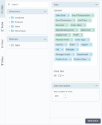
1. On the Data tab, in the Columns field, select the columns for analysis. If all the columns are preselected in the Columns field, remove the ones you do not need. To remove all the columns at once, click the Clear all link in the upper-right corner.

   

   Tip: To select a column, you can click in the field and select it from the list. You can also double-click or drag the columns from the Dimensions and Measures sections on the left. To select multiple columns at once, use the Ctrl or Shift key.

2. If you want to group data by the selected columns, set Group data to On. Otherwise, the data rows are displayed as in the dataset.

3. For large datasets, to improve performance, you can limit the number of rows to explore under Data view options, in the Max number of rows field.

4. Click View data.

   The dataset opens in a tabular view.

In this step, you can profile the columns and evaluate the statistical details of values distribution and frequency of values in selected columns.

1. Click the Profile tab.

2. In the dropdown list, select a column that you want to profile.

   The selected column is pinned as the first column next to the Profile pane for your convenience.

3. Depending on the column type, the following statistics are shown:

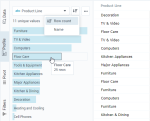
   • Dimensions — All the unique values are listed.

     Point to a value to view the number of rows with this unique value.

     

     You can sort a value by Row count (its frequency) or by Name (alphanumeric).

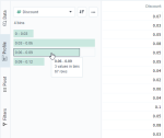
   • Measures — The values are shown in the summary view (in bins) by default.

     Point to a bin to see the number of values in the bin and the number of rows with these values.

     

     To see all the unique values for the selected column, click  More options, and then click Detail view.

     You can sort a value by Row count (its frequency) or by Value (alphanumeric).

   If you need to search for a particular value, you can add a search field (click  More options and click Search).

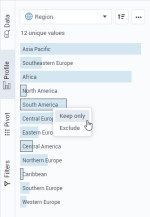
4. To filter data based on the bins or values, right-click the item, and click Keep only or Exclude.

   To select multiple items at once, use the Ctrl or Shift key, and then right-click the selection.

   

   The table is filtered and the filter icon appears next to the column header.

   

In this step, you can reorganize the data to evaluate it from different perspectives.

1. Click the Pivot tab.

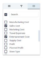
2. Turn on the Pivot Mode, then select the columns that you want to show in the table view. The dimension column names are automatically added to the Rows section and to the top toolbar. The measure column names are automatically added to the Values section. The table data is grouped by default by the dimensions that you selected, in the order in which you selected them.

3. Reorganize your data in several ways:

   • Row grouping

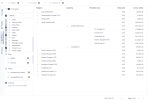
     View the hierarchy of the groups on the toolbar. You can drag the column handles to the left or to the right to rearrange the grouping order or remove columns from grouping.

     

     To add more columns for row grouping, drag the column name handles from the Pivot sidebar to the top toolbar or to the Rows section.

   • Column grouping

     To distribute data vertically by a column, on the sidebar, drag the column handle to the Columns section.

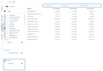
     The values of the selected column appear as new column headers.

     

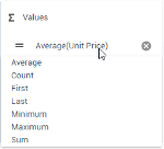
4. To change the aggregation of a measure, click that measure in the Values section, and then select another aggregation type from the dropdown list.

   

In the simple mode (Pivot Mode is off), you can include and exclude columns from the table view, group data by rows, and change aggregation for measures.

In this step, you can apply filters and focus on the data you need.

1. Click the Filters tab.

2. Click the column that you want to filter.

3. Deselect the checkboxes for the values that you want to exclude from the table.

   The data is filtered accordingly and the filter icon appears next to the column name on this tab and in the table.

   

   You can save the filter to the dataset by clicking Save filters to dataset.

   

Review the following topics to learn about table views and capabilities:

Include or exclude columns

Point to a column header, click Options, and then click Columns. Select or deselect checkboxes to show or hide columns in the table. You can start typing in the Filter field to search for a specific column name.

Pin columns

You can set one or more columns to be fixed to the left or right of the table view so that they remain visible when you scroll the table horizontally.

Point to the column header, click Options, then click Pin Column, and select one of the pinning options.

Sort columns

To sort any column, click its header. The arrow appears next to the column name, indicating the sorting order. If no arrow is displayed, the column is not sorted.

Reorder

Drag a column header to the right or to the left to change its order.

Filter data in columns

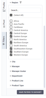
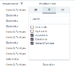
Point to a column header, click Options, and then click the Filters tab (the tab is not available in the grouped columns). Use the list to select or deselect the needed values. After you apply a filter, the filter icon appears next to the column name.

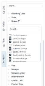
To filter grouped columns, on the sidebar, click the Filters. Click the column that you want to filter, then deselect the checkboxes for the items that you want to exclude from the table. The data is filtered accordingly, and the filter icon appears next to the column name in this tab.

Group rows

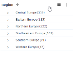
You can organize data in row groups, then collapse and expand the rows to create effective views.

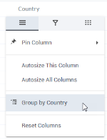
1. Point to the header of a column, click Options, and then click Group by [column name].

   

2. Repeat the same step for adding another level of grouping.

   View the hierarchy of the groups on the toolbar. You can drag column headers to the left or to the right to rearrange the grouping order or remove columns from grouping.

   To expand or collapse all grouped data in a column, point to the column header, click Options and select the corresponding option.

Export data

To export data from a table, right-click anywhere in a row and select one of the following:

• Copy – Copy the current table row and paste it into a document.

  Optionally, to copy a row, you can press Ctrl+C. To select multiple rows, hold Ctrl and click the rows you want to copy. Then, click Copy.

• Copy with Headers – Copy the table row with its column headers.

  To select multiple rows, hold Ctrl and click the rows you want to copy. Then, click Copy with Headers.

• Export – Save the whole table in the following file formats (.csv, .xlsx, or .xml).

The following is an example of the pivot table exported into an Excel file.

References – Column options

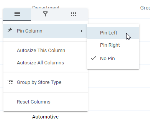
To open the column options menu, point to a column header of the generated table and click Options.

Item	Use this item to
Pin column	Set the column to be fixed to the left or right so that it remains visible when you scroll horizontally to see other columns.
Value aggregation	Change the aggregation of the measures in the grouped rows to one of the following types: Average, Count, First, Last, Minimum, Maximum, or Sum.
Autosize this column	Autosize the current column to the longest value in the column (the header is not considered). Alternatively, you can drag the right border of the column header cell.
Autosize all columns	Autosize all the columns to the longest value in the column (header is not considered).
Group by [column name]	Group the rows by the values in the current column.
Reset columns	Reset the order of the columns, column size, pinned columns, and aggregation to the state in which the table was when you clicked Explore.
Expand all	Expand all row groups. This option appears when you use the grouping option.
Collapse all	Expand all row groups. This option appears when you use the grouping option.